Chapter 6 changes the question we ask about a set. Earlier chapters developed number systems and their operations. We now ask how large a set is, even when there is no last element to count. The answer is expressed through functions: a bijection matches two sets exactly, while an injection records one set inside another without collisions. These ideas make statements about infinite size precise.
Functions used for comparing sets
Let be a function. Its image is
and its preimage of is
The notation can mean the preimage of the singleton ; it does not mean that an inverse function exists. An inverse function exists only when the map is bijective.
Definition
Injection, surjection, and bijection
The function is injective if
Thus every element of has at most one preimage. It is surjective if
or equivalently ; every element of the codomain is hit. It is a bijection if it is both injective and surjective.
The codomain matters. For example, defined by is injective but not surjective because is not hit. If its codomain were , the same rule would be bijective. A claim about cardinality must therefore state both the domain and codomain.
Worked example
Checking the three properties
Consider with
The map is not injective because although . It is not surjective because and are not outputs. This small example separates the two conditions: injectivity concerns repeated outputs, whereas surjectivity concerns omitted codomain elements.
Same cardinality and countability
Definition
Same cardinality
Sets and have the same cardinality, written
if there is a bijection .
The elements being paired need not be alike. A pairing between numbers and ordered pairs is just as legitimate as a pairing between two lists of numbers. For finite sets this agrees with ordinary counting.
Concept lensStructural
Cardinality as counting and as matching
With finite sets, size can feel like an inventory: count the elements. For arbitrary sets, the definition replaces inventory with a matching test: can every element of be paired with exactly one element of , and vice versa? This is why and the even natural numbers have the same cardinality via , even though is a proper subset of . The bijection records equal size; proper containment alone does not imply strictly smaller cardinality.
Definition
Finite set
A set is finite if for some , where we represent by the finite label set ; when , this means . We then write . The empty set is finite, with .
Definition
Countable and at most countable
A set is countable in this course if it is finite or if
Equivalently, it is at most countable when it is finite or countably infinite. Some texts use “countable” only for the infinite case, so the phrase “at most countable” removes that convention ambiguity. A set that is not at most countable is uncountable.
For a countably infinite set, an enumeration is a sequence containing every element exactly once. Saying “exactly once” combines surjectivity of the listing with injectivity of its index map. Merely writing down an infinite sequence is not enough: it must be clear why no element is omitted and why repetitions do not occur.
Explicit countable sets
The integers
Theorem
The integers are countable
.
Assume . Define
This gives the list .
Proof. Every integer is either , a positive integer , or a negative integer with . These occur respectively at index , index , and index . Hence is surjective. The three cases have disjoint values, and within the positive or negative cases the displayed indices determine uniquely, so is injective. Therefore is a bijection. If is indexed from , shift the indices by one; the cardinality statement is unchanged.
This is the basic infinite-set surprise: adding all negative integers to does not create a larger cardinality. The comparison concerns the existence of a bijection, not whether one set contains the other.
The rationals
Theorem
The rationals are countable
The set of rational numbers is at most countable, and in fact countably infinite.
Every positive rational has a unique lowest-terms representation , where and . Put in row and column of a grid. Scan the grid by the finite diagonals . Within each diagonal, scan in increasing numerator (any fixed order would do), and retain only coprime pairs. The beginning is
Worked example
Why the rational diagonal scan works
Take . It is already in lowest terms and lies on the diagonal . Only finitely many diagonals precede diagonal , and diagonal contains only finitely many pairs. Thus is reached at a finite position. Conversely, retaining only coprime pairs means that two recorded pairs cannot represent the same positive rational: uniqueness of lowest terms forces to be the same pair. The scan is therefore both onto and one-to-one.
The same argument explicitly proves both directions. No positive rational is missed because it has a lowest-terms pair, and no positive rational is repeated because that pair is unique. If the resulting list is , then
lists all of exactly once. Zero occurs once, and every nonzero rational has one sign and one positive absolute value. Hence is countable. It is not finite: the inclusion from into is injective, so contains infinitely many distinct integers.
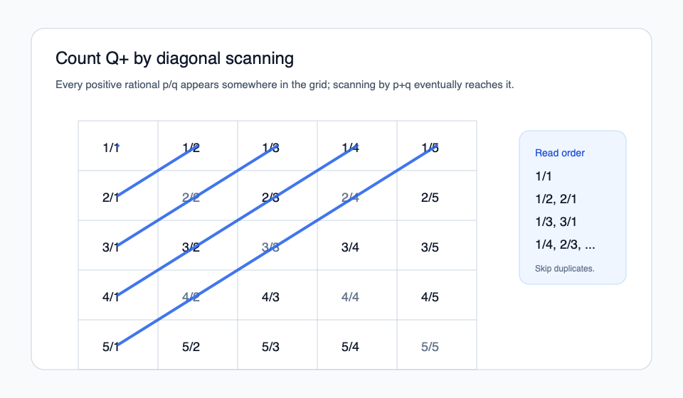
Figure. The diagonal scan turns a two-dimensional grid into one sequence; the lowest-terms condition removes duplicate names for the same rational.
Density is a different property. The rationals meet every nonempty open interval of the real line, but the diagonal procedure still places them in a single list. Dense does not mean uncountable.
Products of countable sets
The grid argument also gives a useful explicit pairing of two copies of . For , let
All pairs with fixed form a finite diagonal, and the triangular number skips exactly the preceding diagonals. Therefore lists every pair once. More formally, from one recovers the unique diagonal satisfying , then and . Thus is a bijection.
Theorem
A countable triple is countable
.
Proof. Define
Both applications of are bijections, so their composition is a bijection from to . The inverse first recovers and then recovers . This is the concrete content of “countable times countable times countable”: a finite-dimensional grid can be scanned by successive finite diagonals. The argument also handles empty factors in the usual way: if one factor is empty, the product is empty and therefore finite; the displayed bijection concerns three copies of .
The same pairing handles a finite number of labelled copies of a countable set. For example, map and into by . The map is injective, so two copies of can be stored in one copy of ; applying the inverse pairing to the appropriate coordinates recovers the label and the original number. This explains why an infinite list can absorb a finite amount of extra bookkeeping. It does not say that every enlargement has the same size: the existence of the particular map must still be proved.
More generally, cardinality comparisons can be transported through maps. If and are injections, their composition gives . If both maps are bijections, the composition is a bijection. These two simple rules are the bookkeeping behind the integer, rational, and triple enumerations in this section.
Cardinal inequalities
Definition
Cardinal inequality
For sets and , write
if there exists an injection . Write if and .
The arrow direction is essential: an injection from into says that has enough distinct locations to store every element of , so the domain is the no-larger side. The inclusion , , proves ; it does not alone prove equality. The enumeration of supplies the reverse size comparison, or the explicit bijection above supplies equality directly.
Worked example
A finite comparison with unused codomain elements
The map given by , , is injective. Thus . It is not surjective because is unused, which is exactly why the inequality may be strict.
Theorem
Cardinal inequalities form a partial-order pattern
The relation is reflexive, transitive, and antisymmetric on cardinalities. Consequently is irreflexive and transitive.
Proof. Reflexivity follows from the injective identity map . For transitivity, if and are injections, then is injective: equality of its outputs first gives equality of the outputs, then equality of inputs. Antisymmetry is precisely the Cantor-Bernstein theorem below. Finally, is impossible because ; transitivity of strict inequality follows by combining transitivity of with the unequal-cardinality conditions.
There is no set whose elements are all sets. Assuming such a universal set would permit a Russell-type self-membership construction and a contradiction. Accordingly, is not being presented as one relation with a global “set of all sets” as its domain. The partial-order statements are about any chosen collection of sets, or the cardinalities represented by that collection, that we are comparing. This qualification is foundational bookkeeping; it does not change any of the maps or proofs above.
A surjection intuitively says that is no larger than , but turning that intuition into an injection requires selecting one preimage for each . The next note examines that choice issue; here we use injections and bijections directly, without assuming a choice function.
Cantor-Bernstein: the two injections fit together
Theorem
Cantor-Bernstein theorem
If and are injections, then .
The theorem is stronger than “two obvious lists look similar.” It constructs a bijection even when neither injection is onto. Set
and recursively define
Because , these sets are nested:
The inclusions are inductive: , then , and the preceding inclusion gives . If or is empty, the two injections force both sets to be empty and the unique empty map is the required bijection; the construction below also covers that case.
The layer is the part on which we will use ; the remaining points lie in and will use the inverse of on its image.
Proof. First note that is injective. For every , it maps bijectively onto . Indeed, injectivity gives one-to-one behavior. If , write with ; if , then , a contradiction. Therefore , proving onto behavior between the layers.
Define by
Here means the inverse of the bijection , not an inverse on all of . The second case is defined: a point outside every layer cannot be in , so it belongs to . The layers are disjoint because they come from a nested sequence, so is well-defined.
To prove injectivity, suppose . If both points lie in layers, injectivity of gives . If both are in the second case, injectivity of gives equality. In the mixed case, say and , the equality implies . The layer mapping just proved puts in , contradicting that was in the second case.
For surjectivity, take and put . If is in no layer, then . Otherwise . It cannot be in the zeroth layer, since while . Hence ; the layer bijection gives an with . Since is injective, , and therefore . Thus is surjective and bijective, proving . No choice function is used: the construction is determined by the given and .
Why coarser layers can miss a point
The sets alone do not record where the inverse of can be used. Put . The first proposed shortcut uses on every difference and on . These pieces exhaust , so that proposal is simply
The second proposal is
Its inverse branch is defined because , but being well-defined does not guarantee a bijection. Take , , and . Then and . Both proposals give , which misses . The layers in the proved construction keep the information these shortcuts discard: where the inverse branch is available and how the two branches avoid collisions.
Common mistakes and subtle points
Common mistake
One injection gives one inequality
An injection proves ; it does not prove equality. For equality, provide a bijection or injections in both directions and invoke Cantor-Bernstein.
Common mistake
Surjective is not the same as injective
A surjection may have many inputs mapping to one output, while an injection may leave codomain elements unused. Always check the correct quantified condition.
Common mistake
Lowest terms are part of the Q proof
Without the coprimality condition, , , and would repeat one rational. The grid is countable, but the proposed list must also be injective.
Checkpoint
Which direction of map proves , and what must it preserve?
State the domain, codomain, and collision condition.
Solution · Answer
An injection proves . It preserves distinctness: forces ; it need not hit every element of .
Checkpoint
Why does the diagonal enumeration list every positive rational?
Use lowest terms and the finite value .
Solution · Answer
Every positive rational has a unique lowest-terms pair . That pair lies on the finite diagonal , and the scan reaches every finite diagonal.
Checkpoint
Why does the Cantor-Bernstein definition use as well as ?
Solution · Answer
ensures that a point outside every layer belongs to , where is defined. Moreover, maps onto . Thus a collision between the two branches would put the point from the inverse branch in a layer, contradicting its branch condition.
Exercises
Checkpoint
Give an explicit bijection from to and prove both injectivity and surjectivity.
Solution · Guided solution
Use , , and for . Zero, each positive integer , and each negative integer appear at indices , , and , respectively, proving surjectivity. These three types of values are disjoint, and each formula determines uniquely, proving injectivity.
Checkpoint
Show directly that using the pairing map .
Solution · Guided solution
First show is bijective by recovering the unique diagonal and then . The composition is a composition of two bijections, hence is a bijection from the triple product to .
Checkpoint
In the Cantor-Bernstein proof, why is defined in the second case?
Solution · Guided solution
The zeroth layer is . A point in no layer is therefore not in that set, so it lies in , where the inverse of is defined.
Related notes
Read 2.2 Functions and relations for images, preimages, injections, surjections, and inverses. Then continue to 6.2 Cantor's theorem, continuum, and choice.